HMAX
Research in the lab is based on a computational model of object recognition in cortex (Riesenhuber & Poggio, Nature Neuroscience, 1999), dubbed HMAX ("Hierarchical Model and X") by Mike Tarr (Nature Neuroscience, 1999) in his News & Views on the paper. Since we didn't think of a better name beforehand, HMAX stuck. Oh well...
The model summarizes the basic facts about the ventral visual stream, a hierarchy of brain areas thought to mediate object recognition in cortex. It was originally developed to account for the experimental data of Logothetis et al. (Cerebral Cortex, 1995) on the invariance properties and shape tuning of neurons in macaque inferotemporal cortex, the highest visual area in the ventral stream. In the meantime, the model has been shown to predict several other experimental results and provide interesting perspectives on still other data and claims. The model is used as a basis in a variety of projects in our and other labs.
The goal is to explain cognitive phenomena in terms of simple and well-understood computational processes in a physiologically plausible model. Thus, the model is a tool to integrate and interpret existing data and to make predictions to guide new experiments. Clearly, the road ahead will require a close interaction between model and experiment. Towards this end, this web site provides background information on HMAX, including the source code, and further references:
Please contact with questions or comments.
Our collaborators in Tommy Poggio's group at MIT have done some really nice work with the model, in particular its application to machine vision problems. Please click here for an overview of their software and papers on the topic (look for "Model of Object Recognition").
The "Standard Model"
Object recognition in cortex is thought to be mediated by the ventral visual pathway (Ungerleider, 1994) running from primary visual cortex, V1, over extrastriate visual areas V2 and V4 to inferotemporal cortex, IT. Based on physiological experiments in monkeys, IT has been postulated to play a central role in object recognition. IT in turn is a major source of input to PFC, "the center of cognitive control" (Miller, 2000) involved in linking perception to memory.
Over the last decades, several physiological studies in non-human primates have established a core of basic facts about cortical mechanisms of recognition that seem to be widely accepted and that confirm and refine older data from neuropsychology. A brief summary of this consensus knowledge begins with the groundbreaking work of Hubel and Wiesel first in the cat (Hubel, 1962, 1965) and then in the macaque (Hubel, 1968). Starting from simple cells in primary visual cortex, V1, with small receptive fields that respond preferably to oriented bars, neurons along the ventral stream (Perrett, 1993; Tanaka, 1996; Logothetis, 1996) show an increase in receptive field size as well as in the complexity of their preferred stimuli (Kobatake, 1994). At the top of the ventral stream, in anterior inferotemporal cortex (AIT), cells are tuned to complex stimuli such as faces (Gross, 1972; Desimone, 1984, 1991; Perrett, 1992). A hallmark of these IT cells is the robustness of their firing to stimulus transformations such as scale and position changes (Tanaka, 1996; Logothetis, 1995, 1996; Perrett, 1993). In addition, as other studies have shown (Perrett, 1993; Booth, 1998; Logothetis, 1995; Hietanen 1992), most neurons show specificity for a certain object view or lighting condition.
A comment about the architecture is important: In its basic, initial operation - akin to "immediate recognition" - the hierarchy is likely to be mainly feedforward (though local feedback loops almost certainly have key roles) (Perrett, 1993). ERP data (Thorpe, 1996) have shown that the process of object recognition appears to take remarkably little time, on the order of the latency of the ventral visual stream (Perrett, 1992), adding to earlier psychophysical studies using a rapid serial visual presentation (RSVP) paradigm (Potter, 1975; Intraub, 1981) that have found that subjects were still able to process images when they were presented as rapidly as 8/s.
In summary, the accumulated evidence points to six mostly accepted properties of the ventral stream architecture:
- A hierarchical build-up of invariances first to position and scale and then to viewpoint and more complex transformations requiring the interpolation between several different object views
- in parallel, an increasing size of the receptive fields
- an increasing complexity of the optimal stimuli for the neurons
- a basic feedforward processing of information (for "immediate" recognition tasks)
- plasticity and learning probably at all stages and certainly at the level of IT
- learning specific to an individual object is not required for scale and position invariance (over a restricted range).
These basic facts lead to a Standard Model, likely to represent the simplest class of models reflecting the known anatomical and biological constraints. It represents in its basic architecture the average belief - often implicit - of many visual physiologists. In this sense it is definitely not "our" model. The broad form of the model is suggested by the basic facts; we have made it quantitative, and thereby predictive (through computer simulations).
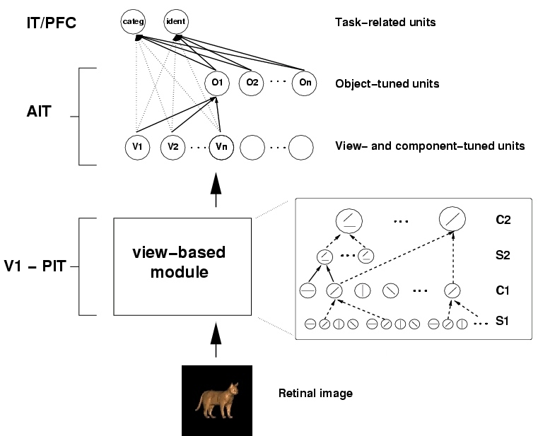
Figure 1: schematic of the Standard Model
The model reflects the general organization of visual cortex in a series of layers from V1 to IT to PFC. From the point of view of invariance properties, it consists of a sequence of two main modules based on two key ideas. The first module, shown schematically above, leads to model units showing the same scale and position invariance properties as the view-tuned IT neurons of (Logothetis, 1995), using the same stimuli. This is not an independent prediction since the model parameters were chosen to fit Logothetis' data. It is, however, not obvious that a hierarchical architecture using plausible neural mechanisms could account for the measured invariance and selectivity. Computationally, this is accomplished by a scheme that can be best explained by taking striate complex cells as an example: invariance to changes in the position of an optimal stimulus (within a range) is obtained in the model by means of a maximum operation (max) performed on the simple cell inputs to the complex cells, where the strongest input determines the cell's output. Simple cell afferents to a complex cell are assumed to have the same preferred orientation with their receptive fields located at different positions. Taking the maximum over the simple cell afferent inputs provides position invariance while preserving feature specificity. The key idea is that the step of filtering followed by a max operation is equivalent to a powerful signal processing technique: select the peak of the correlation between the signal and a given matched filter, where the correlation is either over position or scale. The model alternates layers of units combining simple filters into more complex ones - to increase pattern selectivity with layers based on the max operation - to build invariance to position and scale while preserving pattern selectivity.
In the second part of the architecture, shown above, learning from multiple examples, i.e., different view-tuned neurons, leads to view-invariant units as well as to neural circuits performing specific tasks. The key idea here is that interpolation and generalization can be obtained by simple networks, similar to Gaussian Radial Basis Function networks (Poggio, 1990) that learn from a set of examples, that is, input-output pairs. In this case, inputs are views and the outputs are the parameters of interest such as the label of the object or its pose or expression (for a face). The Gaussian Radial Basis Function (GRBF) network has a hidden unit for each example view, broadly tuned to the features of an example image (see also deBeeck (2001)). The weights from the hidden units to the output are learned from the set of examples, that is input-output pairs. In principle two networks sharing the same hidden units but with different weights (from the hidden units to the output unit), could be trained to perform different tasks such as pose estimation or view-invariant recognition. Depending just on the set of training examples, learning networks of this type can learn to categorize across exemplars of a class (Riesenhuber AI Memo, 2000) as well as to identify an object across different illuminations and different viewpoints. The demonstration (Poggio, 1990) that a view-based GRBF model could achieve view-invariant object recognition in fact motivated psychophysical experiments (Buelthoff, 1992; Gauthier, 1997). In turn the psychophysics provided strong support for the view-based hypothesis against alternative theories (for a review see Tarr (1998)) and, together with the model, triggered the physiological work of Logothetis (1995).
Thus, the two key ideas in the model are:
- the max operation provides invariance at several steps of the hierarchy
- the RBF-like learning network learns a specific task based on a set of cells tuned to example views.
Inside HMAX
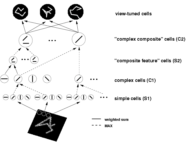
Figure 2: The basic HMAX model consists of a hierarchy of five levels, from the S1 layer with simple-cell like response properties to the VTU level with shape tuning and invariance properties like the view-tuned cells found in monkey inferotemporal cortex (see Logothetis et al., 1995).
For more information, please see the original publications. The basic model is described in the 1999 Nature Neuroscience paper:
Riesenhuber, M. & Poggio, T. (1999). Hierarchical Models of Object Recognition in Cortex. Nature Neuroscience 2: 1019-1025.
More details on how tuning properties, in particular invariance ranges in HMAX depend on pooling parameters, can be found in:
Schneider, R., & Riesenhuber, M. (2004). On the Difficulty of Feature-based Attentional Modulations in Visual Object Recognition: A Modeling Study. CBCL Paper #235/AI Memo #2004‒004, Massachusetts Institute of Technology, Cambridge, MA, February 2004.
S1 Layer
In the HMAX model of object recognition in the ventral visual stream of primates, input images (we used 128 x 128 or 160 x 160 greyscale pixel images) are densely sampled by arrays of two-dimensional Gaussian filters, the so-called S1 units (second derivative of Gaussian, orientations 0°, 45°, 90°, and 135°, sizes from 7 x 7 to 29 x 29 pixels in two-pixel steps) sensitive to bars of different orientations, thus roughly resembling properties of simple cells in striate cortex. At each pixel of the input image, filters of each size and orientation are centered. The filters are sum-normalized to zero and square-normalized to 1, and the result of the convolution of an image patch with a filter is divided by the power (sum of squares) of the image patch. This yields an S1 activity between −1 and 1.
C1 Layer
In the next step, filter bands are defined, i.e., groups of S1 filters of a certain size range (7 x 7 to 9 x 9 pixels; 11 x 11 to 15 x 15 pixels; 17 x 17 to 21 x 21 pixels; and 23 x 23 to 29 x 29 pixels). Within each filter band, a pooling range is defined (variable poolRange) which determines the size of the array of neighboring S1 units of all sizes in that filter band which feed into a C1 unit (roughly corresponding to complex cells of striate cortex). Only S1 filters with the same preferred orientation feed into a given C1 unit to preserve feature specificity. We used pooling range values from 4 for the smallest filters (meaning that 4 x 4 neighboring S1 filters of size 7 x 7 pixels and 4 x 4 filters of size 9x9 pixels feed into a single C1 unit of the smallest filter band) over 6 and 9 for the intermediate filter bands, respectively, to 12 for the largest filter band. The pooling operation that the C1 units use is the "MAX" operation, i.e., a C1 unit's activity is determined by the strongest input it receives. That is, a C1 unit responds best to a bar of the same orientation as the S1 units that feed into it, but already with an amount of spatial and size invariance that corresponds to the spatial and filter size pooling ranges used for a C1 unit in the respective filter band. Additionally, C1 units are invariant to contrast reversal, much as complex cells in striate cortex, by taking the absolute value of their S1 inputs (before performing the MAX operation), modeling input from two sets of simple cell populations with opposite phase. Possible firing rates of a C1 unit thus range from 0 to 1. Furthermore, the receptive fields of the C1 units overlap by a certain amount, given by the value of the parameter c1Overlap. We mostly used a value of 2, meaning that half the S1 units feeding into a C1 unit were also used as input for the adjacent C1 unit in each direction. Higher values of c1Overlap indicate a greater degree of overlap.
S2 Layer
Within each filter band, a square of four adjacent, nonoverlapping C1 units is then grouped to provide input to a S2 unit. There are 256 different types of S2 units in each filter band, corresponding to the 4^4 possible arrangements of four C1 units of each of four types (i.e., preferred bar orientation). The S2 unit response function is a Gaussian with mean 1 (i.e., {1; 1; 1; 1}) and standard deviation 1, i.e., an S2 unit has a maximal firing rate of 1 which is attained if each of its four afferents fires at a rate of 1 as well. S2 units provide the feature dictionary of HMAX, in this case all combinations of 2 x 2 arrangements of "bars" (more precisely, C1 cells) at four possible orientations.
C2 Layer
To finally achieve size invariance over all filter sizes in the four filter bands and position invariance over the whole visual field, the S2 units are again pooled by a MAX operation to yield C2 units, the output units of the HMAX core system, designed to correspond to neurons in extrastriate visual area V4 or posterior IT (PIT). There are 256 C2 units, each of which pools over all S2 units of one type at all positions and scales. Consequently, a C2 unit will fire at the same rate as the most active S2 unit that is selective for the same combination of four bars, but regardless of its scale or position.
VTU Layer
C2 units then again provide input to the viewtuned units (VTUs), named after their property of responding well to a certain two-dimensional view of a three-dimensional object, thereby closely resembling the view-tuned cells found in monkey inferotemporal cortex by Logothetis et al. The C2 to VTU connections are so far the only stage of the HMAX model where learning occurs. A VTU is tuned to a stimulus by selecting the activities of the 256 C2 units in response to that stimulus as the center of a 256-dimensional Gaussian response function, yielding a maximal response of 1 for a VTU in case the C2 activation pattern exactly matches the C2 activation pattern evoked by the training stimulus. To achieve greater robustness in case of cluttered stimulus displays, only those C2 units may be selected as afferents for a VTU that respond most strongly to the training stimulus. An additional parameter specifying response properties of a VTU is its sigma value, or the standard deviation of its Gaussian response function. A smaller sigma value yields more specific tuning since the resultant Gaussian has a narrower half-maximum width.
Source Code
DISCLAIMER OF WARRANTY
The programs provided on this website are provided 'as is' without warranty of any kind. We make no warranties, express or implied, that the programs are free of error, or are consistent with any particular standard of merchantability, or that they will meet your requirements for any particular application. They should not be relied upon for solving a problem whose incorrect solution could result in injury to a person or loss of property. If you do use the programs or procedures in such a manner, it is at your own risk. The authors disclaim all liability for direct, incidental or consequential damages resulting from your use of the programs on this website.
- Function Reference
- Simple Filters
- Standard C/MATLAB Code
- Pure MATLAB Code
- HMAX with Feature Learning
- Modular C++/Matlab Code with Tracing
Function Reference
c2Act = calcCSSITC2new(currClip,[limitPoolFlag])
calcCSSITC2new is the MATLAB function to calculate the C2 responses
(which it returns)
Output
c2Act- C2 activations
Input
currClip- the image (a 2d array) for which to calculate the C2 activity
limitPoolFlag=0- S1 receptive fields are centered at each pixel (in which case the image is zero-padded because some S1 cell receptive fields extend outside the image; this is the original version of the model).
limitPoolFlag=1- C1 activity is only based on S1 cells whose receptive fields lie completely within the image. This parameter is useful if you work with images that have nonzero backgrounds.
Global Variables
filters- holds all S1 simple filters at all possible orientations and all scales
fSiz- holds the sizes of all S1 simple filters, at all possible orientations and all scales
c1SpaceSS- C1 Pooling ranges
c1ScaleSS- S1 Filter ranges
c10L- counts how many C1 cells overlap with each other
s2Sigma- tuning width of C2 units
s2Target- set to 1, this is the target value for S2 cells
Simple Filters
The tarball comes with a filter initialization function, init_filters(whichFilter),
that allows to initialize the following filter types: Second derivative of
a Gaussian (whichFilter='gaussian'): Those are the standard filters,
and the filters used to generate the simulations for the "many feature" version
of the model in the original and subsequent papers. The Methods
section in the 1999 paper erroneously referred to the filters as first derivative
of Gaussian. However, results using first derivative of Gaussian (whichFilter='gaussian1st')
are comparable in terms of VTU selectivity and invariance ranges for the paperclip
benchmark. Gabor filters (whichFilter='gabor') with parameters
chosen to better fit experimental data on V1 simple and complex cell tuning
properties. For more information, see the 2004 AIM Memo.
Standard C/MATLAB Code
This is the standard code that has been used in our papers. Instructions on how to use the C/MATLAB HMAX source code:
- download the HMAX tarball
- untar it: tar -xvf hmax.tar
- do: mex myRespC2new.c (that's the mex function to calculate the C2 activations) to compile the mex .c file into a .mex* or .dll for your platform
- start MATLAB
- type main to run the demo program, which loads in an image (testImage.gray) and calculates the C2 responses for it (which are stored in c2Resp afterwards).
Pure MATLAB Code
has written a pure MATLAB implementation of HMAX that, even though slower than the C/MATLAB hybrid, allows for an easier access/analysis of the intermediate layers of the model.
HMAX with Feature Learning
Thomas Serre has developed a version of HMAX with feature learning (see Serre, Riesenhuber, Louie, & Poggio, 2002) and applied it to face detection.
Modular C++/Matlab Code with Tracing
This code has been contributed by Jim Mutch. We have not tested it in detail and it is not supported by us.
This package is an alternative to the standard HMAX C/MATLAB package. It contains a modular, extensively documented reimplementation of myRespC2new.c which adds a trace option and allows non-square images. The trace option lets you see the location in the image of each C2 unit.
Unlike the original, this version explicitly computes and stores each layer. This takes more memory, but permits a more modular program structure. This simplified debugging and addition of the trace option, and should be easier for others to understand and modify.
This implementation also tightens up a few boundary conditions affecting the number of intermediate-level units for images of various sizes. For this reason, the outputs will not exactly match those of the standard C/MATLAB package.
Note that this version uses filters of the Gaussian first derivative in the 'main.m' example. Hence the results will differ from the default 'main' in the C/Matlab package which uses the second derivative.
Instructions:
- Download ModularHMAXWithTracing.tar into its own directory
- Untar it with the command tar -xvf ModularHMAXWithTracing.tar
- Follow the instructions in ReadMe.txt
Note also that while the code uses a few convenient C++ features (bool type, passing by reference), it is otherwise pure C, and not object-oriented.
Publications
This list is a little outdated; for the latest, see the main publications page.
Journal Papers
- Riesenhuber, M., & Poggio, T. (2002). Neural Mechanisms of Object Recognition.
Current Opinion in Neurobiology 12: 162-168.
[ the latest review ] - Riesenhuber, M. & Poggio, T. (2000). Models of Object Recognition. Nature Neuroscience 3(supp.): 1199-1204.
- Riesenhuber, M. & Poggio, T. (1999). Hierarchical
Models of Object Recognition in Cortex. Nature Neuroscience
2: 1019-1025.
[postscript | gzipped postscript] [supplement: postscript | gzipped postscript]
The original HMAX paper (see also News and Views by Mike Tarr below) - Riesenhuber, M. & Poggio, T. (1999).
Are Cortical Models Really Bound by the 'Binding Problem'? Neuron
24: 87-93.
[postscript | gzipped postscript]
Technical Reports
- Schneider, R., & Riesenhuber, M. (2003). A Detailed Look at Scale and Translation Invariance in a Hierarchical Neural Model of Visual Object Recognition. CBCL Paper #218/AI Memo #2002‒011, Massachusetts Institute of Technology, Cambridge, MA, August 2002.
- Knoblich, U., Freedman, D.J., Riesenhuber, M. (2002). Categorization in IT and PFC: Model and Experiments. CBCL Paper #216/AI Memo #2002‒007, Massachusetts Institute of Technology, Cambridge, MA, April 2002.
- Knoblich, U. & Riesenhuber, M. (2002). Stimulus Simplification and Object Representation: A Modeling Study. CBCL Paper #215/AI Memo #2002‒004, Massachusetts Institute of Technology, Cambridge, MA, March 2002.
- Riesenhuber, M. Generalization Over Contrast and Mirror Reversal, but Not Figure-ground Reversal, in an "Edge-based" Model of IT Neurons. CBCL Paper #211/AI Memo #2001‒034, Massachusetts Institute of Technology, Cambridge, MA, December 2001.
- Riesenhuber, M., & Poggio, T. (2000).
The Individual is Nothing, the Class Everything: Psychophysics and Modeling
of Recognition in Object Classes. AI Memo 1682, CBCL Paper 185, Artificial
Intelligence Lab and Center for Biological & Computational Learning,
Massachusetts Institute of Technology.
[ postscript | gzipped postscript ] - Riesenhuber, M., & Poggio, T. (1999). A Note on Object Class Representation and Categorical Perception. AI Memo 1679, CBCL Paper 183, Artificial Intelligence Lab and Center for Biological & Computational Learning, Massachusetts Institute of Technology.
- Riesenhuber, M., & Poggio, T. (1998). Modeling Invariances in Inferotemporal Cell Tuning. AI Memo 1629, CBCL Paper 160, Artificial Intelligence Lab and Center for Biological & Computational Learning, Massachusetts Institute of Technology.
Conference Papers
- Knoblich, U., Riesenhuber, M., Freedman, D.J., Miller, E.K., & Poggio, T. (2002). Visual Categorization: How the Monkey Brain Does It. In Biologically Motivated Computer Vision, Lee, S-W., H.H. Buelthoff & T. Poggio (eds.), Second IEEE International Workshop, BMCV 2002, Tuebingen, Germany, December 2002, 273-281.
- Serre, T., Riesenhuber, M., Louie, J., & Poggio, T. (2002). On the Role of Object-Specific Features for Real World Object Recognition in Biological Vision. In Biologically Motivated Computer Vision, Lee, S-W., H.H. Buelthoff & T. Poggio (eds.), Second IEEE International Workshop, BMCV 2002, Tuebingen, Germany, December 2002, 387-397.
- Walther, D., Itti, L., Riesenhuber, M., Poggio, T., & Koch, C. (2002). Attentional Selection for Object Recognition - A Gentle Way. In Biologically Motivated Computer Vision, Lee, S-W., H.H. Buelthoff & T. Poggio (eds.), Second IEEE International Workshop, BMCV 2002, Tuebingen, Germany, December 2002, 472-479.
- Riesenhuber, M., & Poggio, T. (2000). CBF: A New Framework for Object Categorization in Cortex. In Biologically Motivated Computer Vision, Lee, S-W., H.H. Buelthoff & T. Poggio (eds.), First IEEE International Workshop, BMCV 2000, Seoul, Korea, May 2000.
- Riesenhuber, M., & Poggio, T. (1998). Just One View: Invariances in Inferotemporal Cell Tuning. In Advances in Neural Information Processing Systems 10, 215-221. MIT Press.
Experimental Papers
Experimental papers testing model hypotheses:
- Freedman, D.J., Riesenhuber, M., Poggio, T., & Miller, E.K. (2003). A Comparison of Primate Prefrontal and Inferior Temporal Cortices during Visual Categorization. Journal of Neuroscience 23, 5235-5246.
- Gawne, T. & Martin, J. (2002). Responses of primate visual cortical V4 neurons to simultaneously presented stimuli. Journal of Neurophysiology 88: 1128-1135.
Related Papers
Related papers and commentary:
- Rousselet, G.A., Thorpe, S.J., & Fabre-Thorpe, M. (2003). Taking the MAX from neuronal responses. Trends in Cognitive Sciences 7: 99-102.
- Tarr, M. (1999). News and Views: Pandemonium Revisited. Nature Neuroscience 2: 932-935.